

Overview
The latest HMC-Sim 3.0 branch development has included the ability to record basic, functional power and thermal tracing across each the sub-device components on each clock cycle. The tracing data can be written to the default trace output file or to Tecplot files. This tutorial provides users with a better understanding of configuring and utilizing the power/thermal trace data. We will also provide details on generating 3D visualization content using the generated Tecplot output. For more information on the basic power/thermal functionality, refer to the HMC-Sim page and the CMC tutorial.
HMC-Sim Power/Thermal Component Configuration
As noted in the HMC-Sim development page, the sub-device component power tracing (and the associated thermal tracing) are based upon a default set of values hard coded into the simulation infrastructure. However, users have the ability to modify these values at will based upon the target simulated device configuration. Modifying the simulation values can be accomplished using two methods.
First, the HMC-Sim 3.0 branch development includes an additional user-facing function interface that provides users the ability to manually instantiate the individual sub-device component power values. These values represent the power required to service the respective sub-device component on a single clock cycle (or full row cycle in the case of the DRAM row access power). The function interface accepts floating point values in milliwatts for each of the sub-device component power values. The function returns 0 on success and nonzero otherwise. The function interface is defined as follows:
extern int hmcsim_power_config( struct hmcsim_t *hmc,
 float link_phy,
 float link_local_route,
 float link_remote_route,
 float xbar_rqst_slot,
 float xbar_rsp_slot,
 float xbar_route_extern,
 float vault_rqst_slot,
 float vault_rsp_slot,
 float vault_ctrl,
 float row_access );
In addition to the aforementioned function interface, the HMC-Sim 3.0 development branch also provides the ability to initialize the sub-device component power configuration values from a configuration file. This method also requires the use of an additional function interface, but provides users the ability to reuse the configuration file across multiple instantiations of the simulator. Further, the configuration method is currently the only route by which to enable Tecplot trace output for 3D visualization.
First, the configuration file function interface is defined as follows (where ‘config’ contains the filename of the target configuration file):
extern int hmcsim_read_config( struct hmcsim_t *hmc, char *config );
The configuration files accept basic KEYWORD = VALUE where blank lines are ignored and lines beginning with ‘#’ are considered comments. The configuration file values are outlined in the following table:
| Configuration Value | Type | Description |
|---|---|---|
| LINK_PHY_POWER | Float | Link phy power (milliwatts) |
| LINK_LOCAL_ROUTE_POWER | Float | Link local route (phy to locally connected quad) power (milliwatts) |
| LINK_REMOTE_ROUTE_POWER | Float | Link remote route (phy to remotely connected quad) power (milliwatts) |
| XBAR_RQST_SLOT_POWER | Float | Crossbar request slot power (milliwatts) |
| XBAR_RSP_SLOT_POWER | Float | Crossbar response slot power (milliwatts) |
| XBAR_ROUTE_EXTERN_POWER | Float | Crossbar route to externally connected link (cube to cube) power (milliwatts) |
| VAULT_RQST_SLOT_POWER | Float | Vault request slot power (milliwatts) |
| VAULT_RSP_SLOT_POWER | Float | Vault response slot power (milliwatts) |
| VAULT_CTRL_POWER | Float | Vault controller power (milliwatts) |
| ROW_ACCESS_POWER | Float | Row access power (entire dram row fetch, milliwatts) |
| TECPLOT_OUTPUT | {0,1} | Toggles tecplot output; 0=disabled; 1=enabled Enabling will create a tecplot file for each clock cycle for power and thermal output |
| TECPLOT_PREFIX | String (1024 characters) | Tecplot file prefix; Forces tecplot output to: PREFIX-power.CLOCK.tec PREFIX-therm.CLOCK.tec |
A sample configuration file is as follows:
# config.sample
# configuration file to setup power measurement values

LINK_PHY_POWER = 10

LINK_LOCAL_ROUTE_POWER = 20

LINK_REMOTE_ROUTE_POWER = 30

XBAR_RQST_SLOT_POWER = 2

XBAR_RSP_SLOT_POWER = 2.5

XBAR_ROUTE_EXTERN_POWER = 35

VAULT_RQST_SLOT_POWER = 27

VAULT_RSP_SLOT_POWER = 21

VAULT_CTRL_POWER = 5

ROW_ACCESS_POWER = 17

TECPLOT_OUTPUT = 1

TECPLOT_PREFIX = STREAM
HMC-Sim Power/Thermal Visualization
As mentioned above, the latest development branch of HMC-Sim includes the ability to output Tecplot-style trace data. The Tecplot output files are not designed to be human readable. Rather, they are designed to be imported into one or more 3D visualization tools/applications such that users can visually represent the power and thermal output data.
In order to utilize this feature in HMC-Sim, you must utilize the power configuration files mentioned in the previous section. Setting the TECPLOT_OUTPUT keyword to “1” will enable the default output tracing. It is also highly recommended to set a preferred output file prefix using TECPLOT_PREFIX. This will ensure that the files are properly named as follows: PREFIX-{power,therm}.CLOCK.tec.
Using these configuration values, HMC-Sim will output two sets of Tecplot files for each clock cycle. The *-power files contain the power data for each sub-device component organized in a 3D cubic structure for the respective clock cycle. The *-therm files contain the thermal data for each sub-device component in the same 3D cubic structure for the respective clock cycle. Please note, given that the simulator will output two files for every clock cycle, please be aware of any file system limitations that may prevent the creation of a large number of files for long-running simulations. For example, if your simulation executes for 2,000 cycles, HMC-Sim will create 4,000 Tecplot files in the current working directory.
Once you successfully complete your simulation run and create the aforementioned Tecplot output files, you can import these into several target visualization applications/tools. For the purpose of this tutorial, we utilize the VisIt application developed and distributed by the US Department of Energy. Refer to the VisIt users website for more information regarding installation and best practices for users.
This tutorial was originally developed using VisIt 2.12 on Mac OSX 10.11.6. We assume that the user has installed and successfully tested their respective VisIt installation.
Note: Click on any of the images to view a larger version.
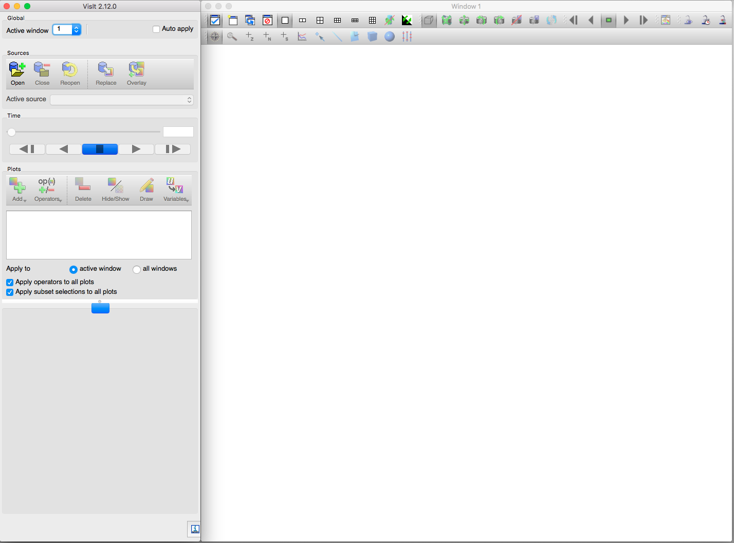
Step 1: Open the VisIt application
The first step in the process of creating our output visualization is to open VisIt. VisIt should open with a blank canvas and a series of toolbars as follows:
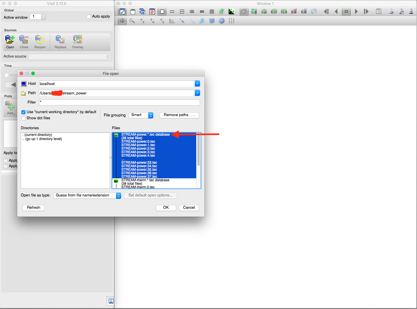
Step 2: Open Tecplot Data Set
Now that the application is open, we need to open one of our Tecplot output sets. This can be either the power output data or the thermal (therm) output data. In order to do so, select the File->Open File menu item. This will open a dialog box. Browse to the location of our Tecplot output files in the left pane. Select the corresponding *.TEC entry, which is subsequently highlight the entire block of Tecplot files. This will import the entire Tecplot “database” into VisIt for use as the input for our visualization.
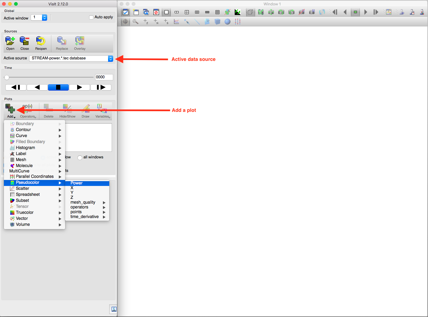
Step 3: Add a Pseudocolor Plot
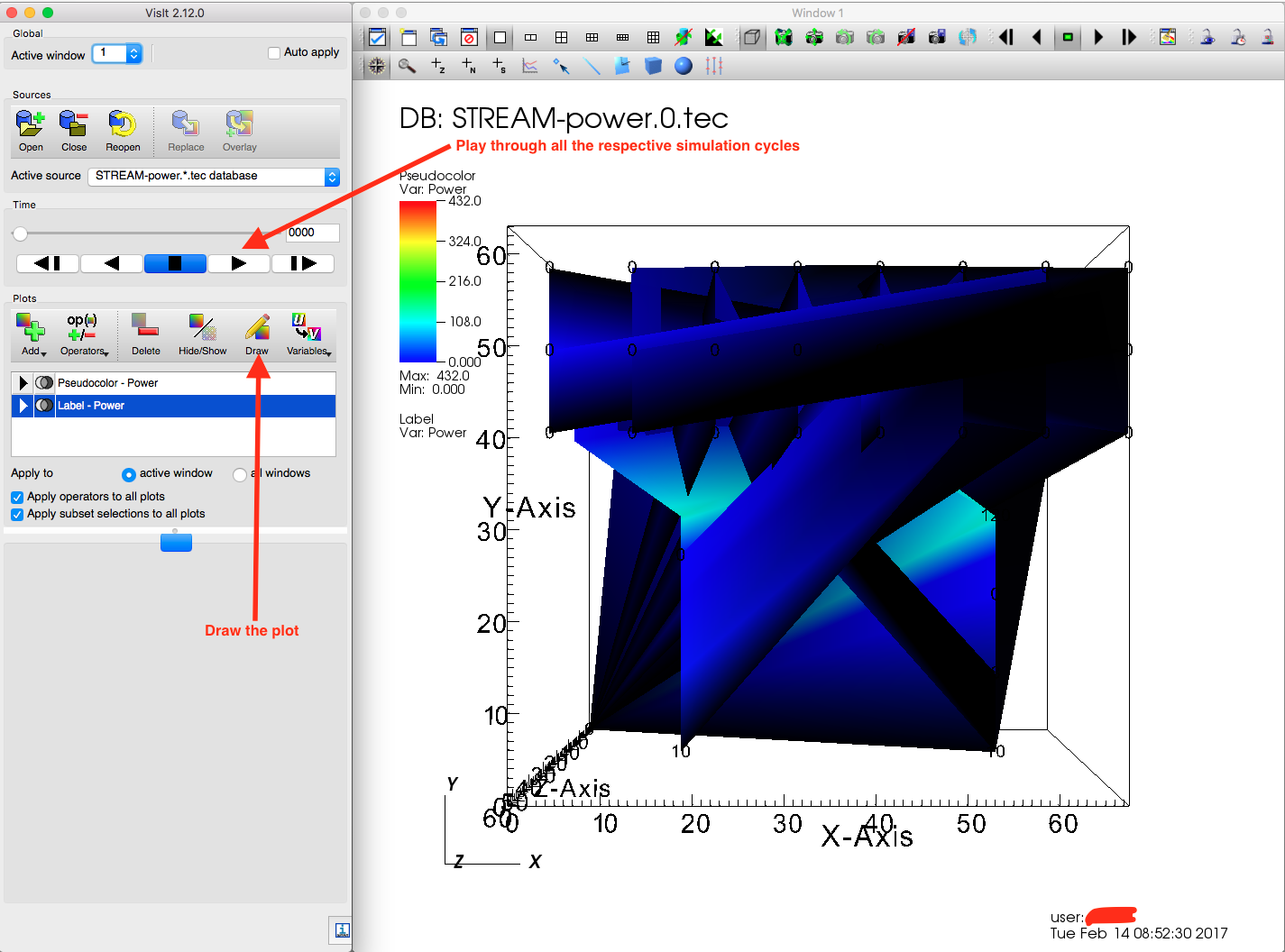
Now that we have our source data open, we should see it as an active data source (see the figure below). Now we can begin adding visualization plots based upon the input set. In the left pane of VisIt under “Plots”, we want to select Add->Pseudocolor->Power (If the *-therm data was opened, we would select “BTU” instead). This will create a three dimensional cubic structure of our plot data whereby the power (or thermal) values a represented as colors. Larger numbers indicating higher power or thermal density will be represented in reds or orange colors. Lower power states are represented as cooler colors such as blue and violet.
Note that selecting the plot will not immediately display any visualization data. You must also select the Draw button under the same “Plots” pane to view the visualization data as a rendered entity.
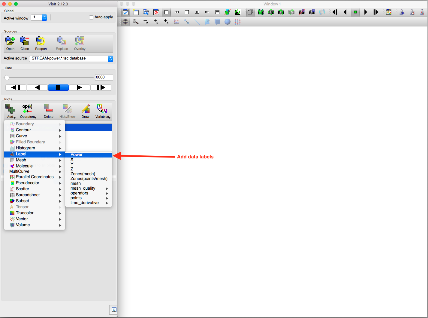
Step 4: [Optional] Add Data Labels
You may also add the intermediate data labels to our plot. This will label the respective areas within the 3D space with their respective data labels for each unique clock cycle. This can be accomplished by selecting the Add->Label->Power (or BTU) in the same “Plots” pane.
Step 5: Draw (render) the Visualization
Now that we have all the respective data imported and the correct set of plots selected, we can draw (render) the visualization. This can be accomplished by selecting the Draw button under “Plots” pane. Immediately above the “Plots” pane is in the “Time” pane. Within this application pane are a series of buttons to advance or retreat in simulation time. We can also play through the entire simulation. For each clock cycle, the data will be updated per the respective Tecplot input. You can also manipulate the position of the 3D cube by clicking, holding and dragging up/down/left/right. Refer to the VisIt user documentation for more information on manipulating the visual aspects of the plot.
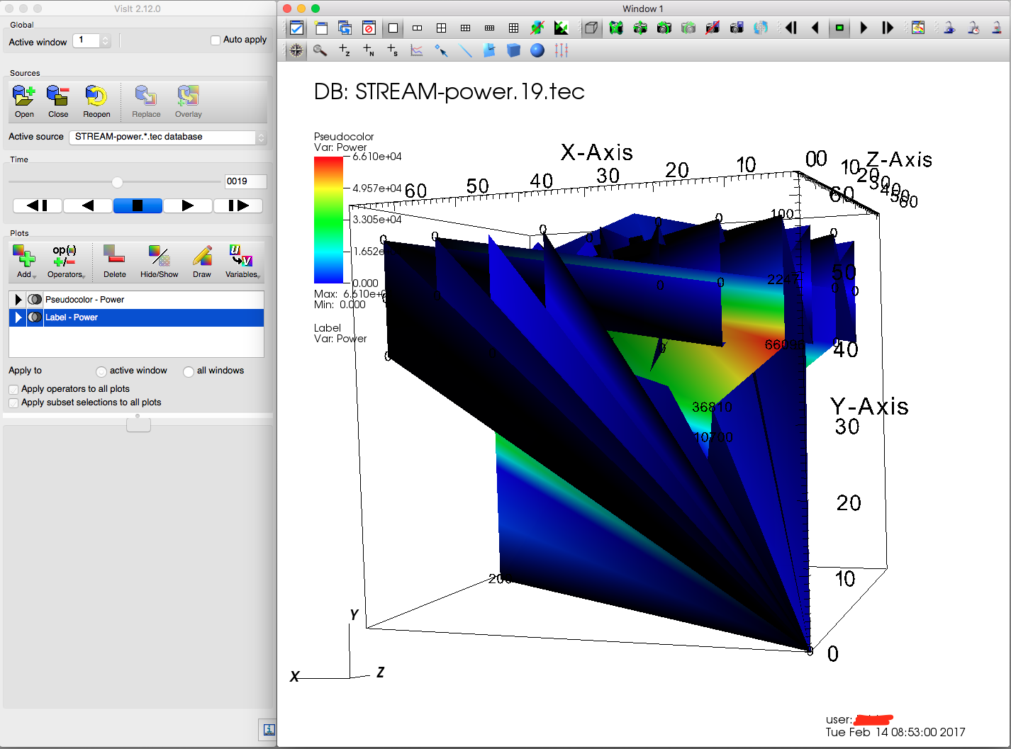
The arrangement of the sub-device components in the 3D space is designed to mimic the actual HMC device layout. The lowest Y values represent the physical links. The next layer represents the crossbar queues and the crossbar routing. The next layer represents the vault queues. The upper most layer is the DRAM region.
Rotated visualization
Step 6: Render Full Movie
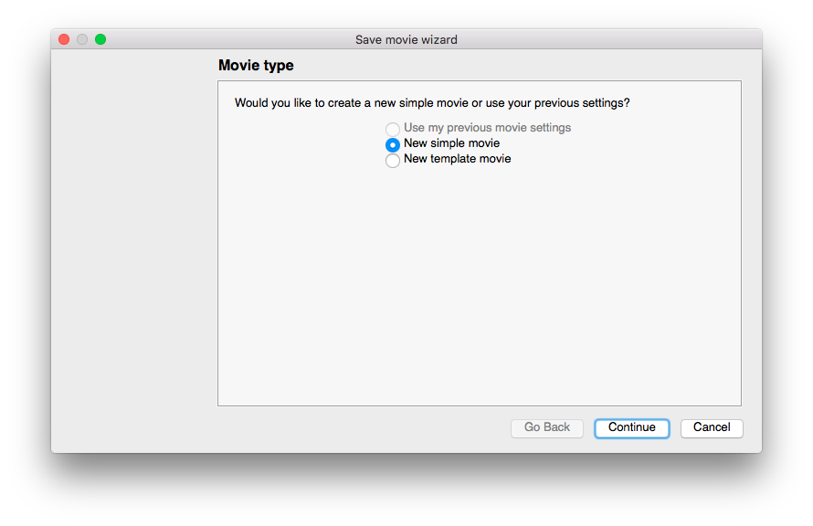
Now that we have our visualization imported and rendered, we can optionally create a full video that includes all the rendered frames of the set. This can be done by selecting the File->Save Movie menu item, which subsequently opens a series of dialog boxes. In the first dialog box, we select “New simple move” and click Continue.
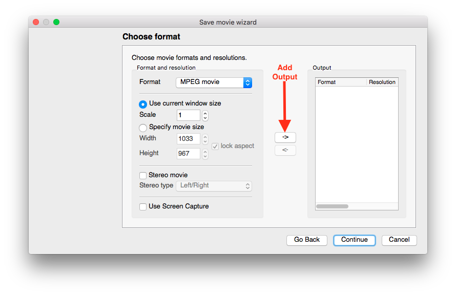
The next dialog permits us to modify the output file type (encoding) and the size (XY dimensions) of the video. We leave these as default, but users can modify at will. In order to complete the action, you need to select the right arrow button to add the output details as a render output. Once this is complete, click Continue.
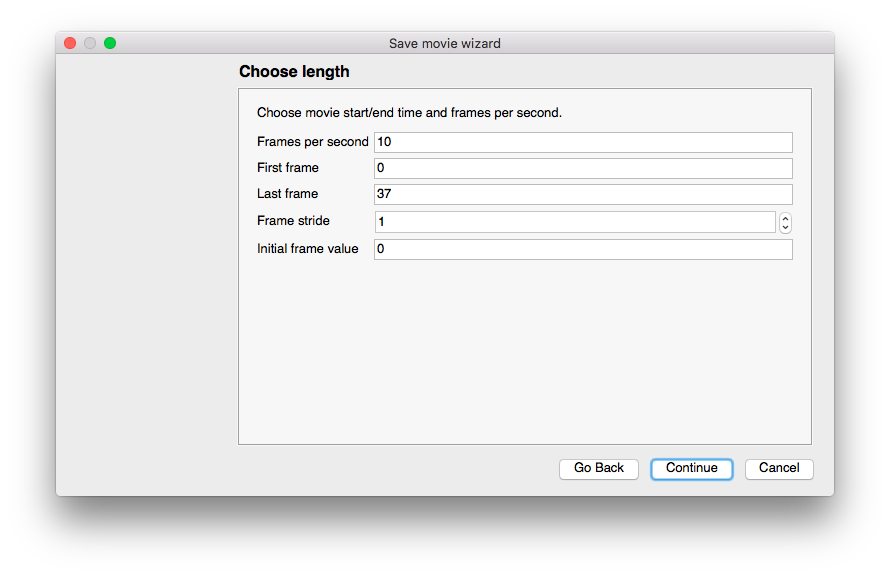
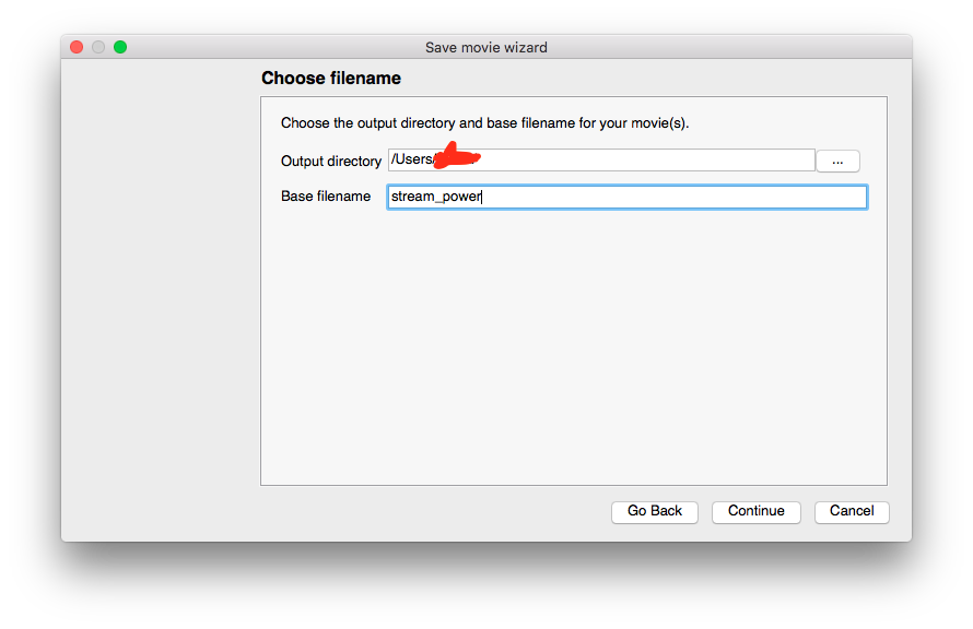
The next dialog screen permits us to select the starting/ending frame, the frame-rate and other details of the video progression. We leave these as default values. The following dialog permits us to select an appropriate output directory and a filename prefix.
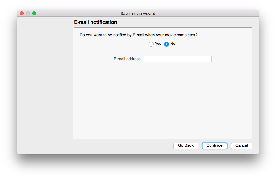
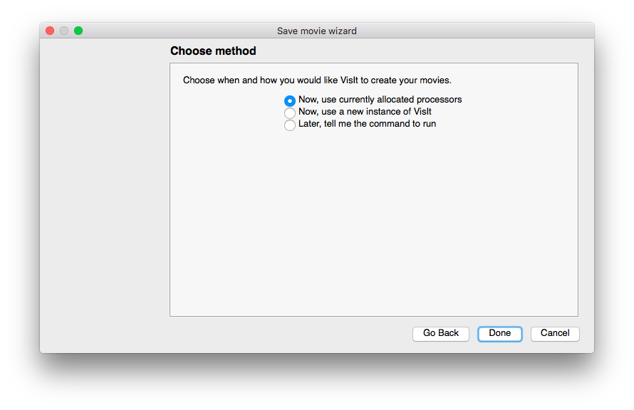
The next dialog prompts us to determine whether the system should email us when the rendering is complete. This is only really useful for visualizations that include a large number of inputs (Tecplot files). The final dialog prompts us for the timing and number of processors to utilize for the render job. We generally leave the default values in both of these dialog boxes.
We present a pair of sample visualization videos in the following section.
HMC-Sim Sample Visualizations
These visualizations were created from the STREAM_POWER_TECPLOT sample test located in the gc64-hmcsim/test directory.